Simulates C3 photosynthesis

Usage

c3photo(Qp, Tl, RH, vcmax = 100, jmax = 180, Rd = 1.1, Catm = 380, O2 = 210, b0 = 0.08, b1 = 5, theta = 0.7, StomWS = 1, ws = c("gs", "vmax"))

Arguments

Qp

Quantum flux

Tl

Leaf temperature

RH

Relative humidity (fraction -- 0-1)

vcmax

Maximum rate of carboxylation

jmax

Maximum rate of electron transport

Rd

Leaf dark respiration

Catm

Atmospheric carbon dioxide.

O2

Atmospheric Oxygen concentration (mmol/mol)

b0

Intercept for the Ball-Berry model

b1

Slope for the Ball-Berry model

theta

Curvature parameter

Examples

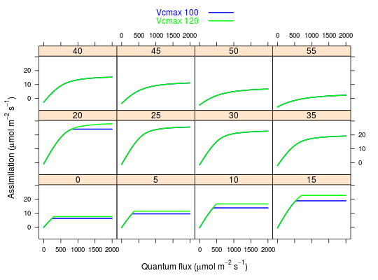
## Testing the c3photo function
## First example: looking at the effect of changing Vcmax
Qps <- seq(0,2000,10)
Tls <- seq(0,55,5)
rhs <- c(0.7)
dat1 <- data.frame(expand.grid(Qp=Qps,Tl=Tls,RH=rhs))

res1 <- c3photo(dat1$Qp,dat1$Tl,dat1$RH) ## default Vcmax = 100
res2 <- c3photo(dat1$Qp,dat1$Tl,dat1$RH,vcmax=120)

## Plot comparing alpha 0.04 vs. 0.06 for a range of conditions
xyplot(res1$Assim + res2$Assim ~ Qp | factor(Tl) , data = dat1,
            type='l',col=c('blue','green'),lwd=2,
            ylab=expression(paste('Assimilation (',
                 mu,mol,' ',m^-2,' ',s^-1,')')),
             xlab=expression(paste('Quantum flux (',
                 mu,mol,' ',m^-2,' ',s^-1,')')),
            key=list(text=list(c('Vcmax 100','Vcmax 120')),
              lines=TRUE,col=c('blue','green'),lwd=2))



## Second example: looking at the effect of changing Jmax
## Plot comparing Jmax 300 vs. 100 for a range of conditions

res1 <- c3photo(dat1$Qp,dat1$Tl,dat1$RH) ## default Jmax = 300
res2 <- c3photo(dat1$Qp,dat1$Tl,dat1$RH,jmax=100)

xyplot(res1$Assim + res2$Assim ~ Qp | factor(Tl) , data = dat1,
           type='l',col=c('blue','green'),lwd=2,
            ylab=expression(paste('Assimilation (',
                 mu,mol,' ',m^-2,' ',s^-1,')')),
             xlab=expression(paste('Quantum flux (',
                 mu,mol,' ',m^-2,' ',s^-1,')')),
            key=list(text=list(c('Jmax 300','Jmax 100')),
              lines=TRUE,col=c('blue','green'),lwd=2))



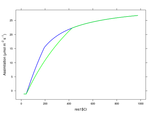
## A/Ci curve

Ca <- seq(20,1000,length.out=50)
dat2 <- data.frame(Qp=rep(700,50), Tl=rep(25,50), rh=rep(0.7,50))
res1 <- c3photo(dat2$Qp, dat2$Tl, dat2$rh, Catm = Ca)
res2 <- c3photo(dat2$Qp, dat2$Tl, dat2$rh, Catm = Ca, vcmax = 70)

xyplot(res1$Assim ~ res1$Ci,
           lwd=2,
           panel = function(x,y,...){
                   panel.xyplot(x,y,type='l',col='blue',...)
                   panel.xyplot(res2$Ci,res2$Assim, type='l', col =
           'green',...)
           },
            ylab=expression(paste('Assimilation (',
                 mu,mol,' ',m^-2,' ',s^-1,')')))

See also

Author